Hey Friends,
In my previous post, I wrote about Data Analysis toolpack in Excel. In this post, I would like to share with you how can you create powerful and interactive maps out of the data you have using Google Sheets.
If you are a Sales & Marketing professional, you might need this functionality in order to get a visual representation of the locations of your clients or customers or the amount of revenue generated from each geographic region. Possibilities are endless, anyone can use this feature for their respective data representation task which involves geographic region.
In this post, I have used Google Sheets instead of MS Excel because MS Excel supports Geo Chart functionality only in a few higher versions, which I am currently not using. Hence it's time to use Google Sheets!
Let us get started with creating a geographical representation of our data.
Step 1:
Go to Google Sheet by clicking on this link or typing it in your browser
https://docs.google.com/spreadsheets/u/0/
Step 2:
Now start by creating a New Blank spreadsheet
Step 3:
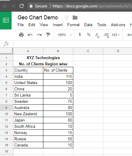
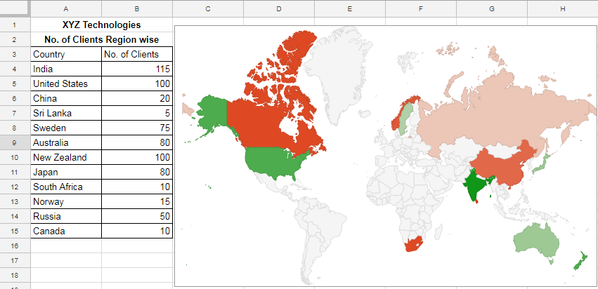
Enter your data into the cells with country names in one column and other numeric figures in an another column. For your reference, you can use the sample data as shown in the image below:
While entering the Country names, make sure you avoid making any typographical or spelling errors. While playing with this, I have noticed that Google's intelligent engine is able to identify the country to certain extent even in case we make some errors. That's the power of Intelligent Google!
In my previous post, I wrote about Data Analysis toolpack in Excel. In this post, I would like to share with you how can you create powerful and interactive maps out of the data you have using Google Sheets.
If you are a Sales & Marketing professional, you might need this functionality in order to get a visual representation of the locations of your clients or customers or the amount of revenue generated from each geographic region. Possibilities are endless, anyone can use this feature for their respective data representation task which involves geographic region.
In this post, I have used Google Sheets instead of MS Excel because MS Excel supports Geo Chart functionality only in a few higher versions, which I am currently not using. Hence it's time to use Google Sheets!
Let us get started with creating a geographical representation of our data.
Step 1:
Go to Google Sheet by clicking on this link or typing it in your browser
https://docs.google.com/spreadsheets/u/0/
Step 2:
Now start by creating a New Blank spreadsheet
Step 3:
Enter your data into the cells with country names in one column and other numeric figures in an another column. For your reference, you can use the sample data as shown in the image below:
|
| Sample Data for Geo Chart Demo |
While entering the Country names, make sure you avoid making any typographical or spelling errors. While playing with this, I have noticed that Google's intelligent engine is able to identify the country to certain extent even in case we make some errors. That's the power of Intelligent Google!
Step 4:
Now select the complete table with both the country column & the numeric column
and click on Insert > Chart from the menu bar or alternatively from the
toolbar using the Chart icon.
Voila! The Chart Dialog box would open up as shown in the below image:

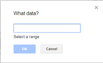
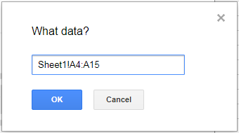
Now click on the field area and select a range of cells containing the names of the country. In this case select from India to Canada. (Do not include header titles of the column since we have unchecked that option.)
The dialog box would appear like this. Click OK.


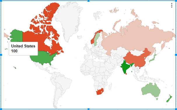
As I said in the beginning of my post, these charts are Interactive. Hence you can click inside the chart area and hover over any geographic region, you would be able to see the numeric value associated with that region as shown below:
Apart from this chart, Google sheet also provide another map called "Geo Charts with Markers". You can use that by selecting the same option from "Chart Type" drop down menu. For the same table data, the corresponding Marker Geo chart would look like the following:
Voila! The Chart Dialog box would open up as shown in the below image:
Step 5:
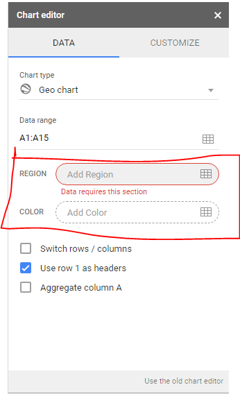
Now from "Chart Type" drop down menu, select "Map" or "Geo Chart".
Now the dialog box would change as shown in the below image.
Most of the time the chart will auto populate the field by automatically
guessing and ignoring the column headings. If in your case, the map didn't
appear, you can follow the further steps.
Step 6:
Uncheck the option "Use row 1 as headers". This is because we would be
selecting only cell values instead of selecting them along with their
respective column headers in the upcoming steps.
Now we have to enter the cell locations at 2 fields.
REGION - Here, We need to enter the address of the cell locations wherein
the country names have been entered. Click on the table icon shown on the right
side of field, a dialog box would appear as shown below
Now click on the field area and select a range of cells containing the names of the country. In this case select from India to Canada. (Do not include header titles of the column since we have unchecked that option.)
The dialog box would appear like this. Click OK.
COLOR - Now, In this field we need to enter the address of the range of
numeric values associated with each geographical region. Follow the same steps
which we followed for "Region" field.
Now the dialog box would appear as follows:
If you have completed till this step, you would see the Geographical map chart
as shown below:
As I said in the beginning of my post, these charts are Interactive. Hence you can click inside the chart area and hover over any geographic region, you would be able to see the numeric value associated with that region as shown below:
|
| Geo Chart |
Apart from this chart, Google sheet also provide another map called "Geo Charts with Markers". You can use that by selecting the same option from "Chart Type" drop down menu. For the same table data, the corresponding Marker Geo chart would look like the following:

|
| Geo Chart with Markers |
I know the previous chart looks better :) But you can still play around with the
numeric values and check out which appears better for your data.
I hope this post was helpful. Do check out my other posts on Google Sheets &
Excel.